ranger - Random Forest • vivid

This guide is designed as a quick-stop reference of how to use some of the more popular machine learning R packages with vivid. In the following examples, we use the air quality data for regression and the iris data for classification.

library('vivid')
library("ranger")

ranger - Random Forest

The ranger package in R is a fast implementation of Random Forests, leveraging optimized C++ code for efficiency.

Regression

# load data
aq <- na.omit(airquality)

# build rf model
rf <- ranger(Ozone ~ ., data = aq)

# vivid
vi <- vivi(data = aq, fit = rf, response = 'Ozone')

Heatmap

viviHeatmap(mat = vi)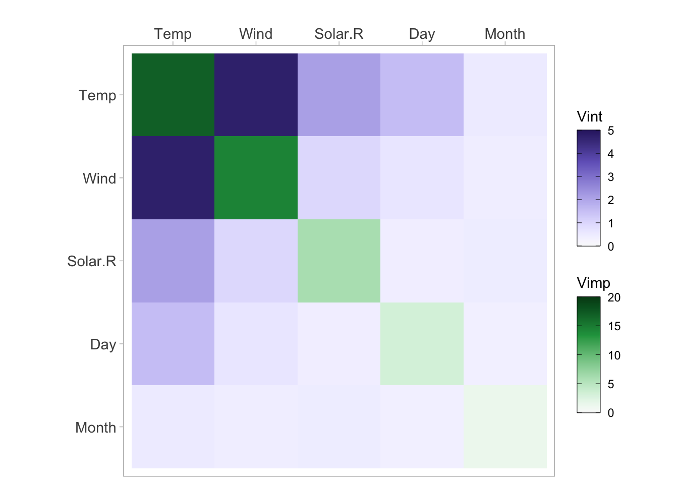

Figure 1: Heatmap of a ranger random forest regression fit displaying 2-way interaction strength on the off diagonal and individual variable importance on the diagonal.

PDP

pdpPairs(data = aq, 
         fit =  rf, 
         response = "Ozone", 
         nmax = 500, 
         gridSize = 20,         
         nIce = 100)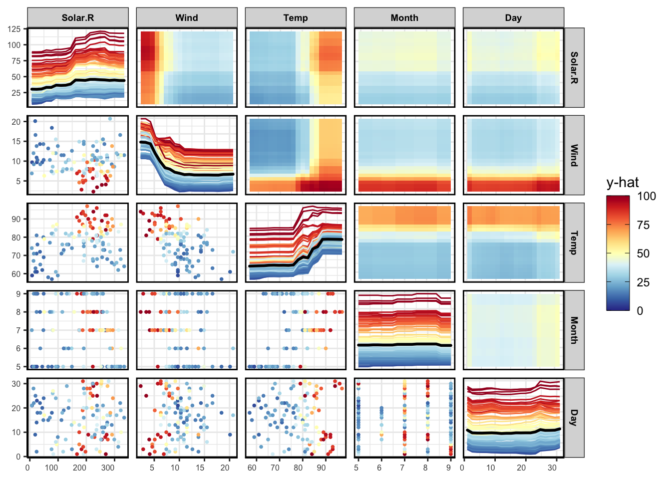

Figure 2: Generalized pairs partial dependence plot for a ranger random forest regression fit.

Classification


# Load the iris dataset
data(iris)

# Train 
rf <- ranger(Species ~ ., data = iris, probability = T)

vi <- vivi(data = iris, fit = rf, response = 'Species', class = 'setosa')

Heatmap

viviHeatmap(mat = vi)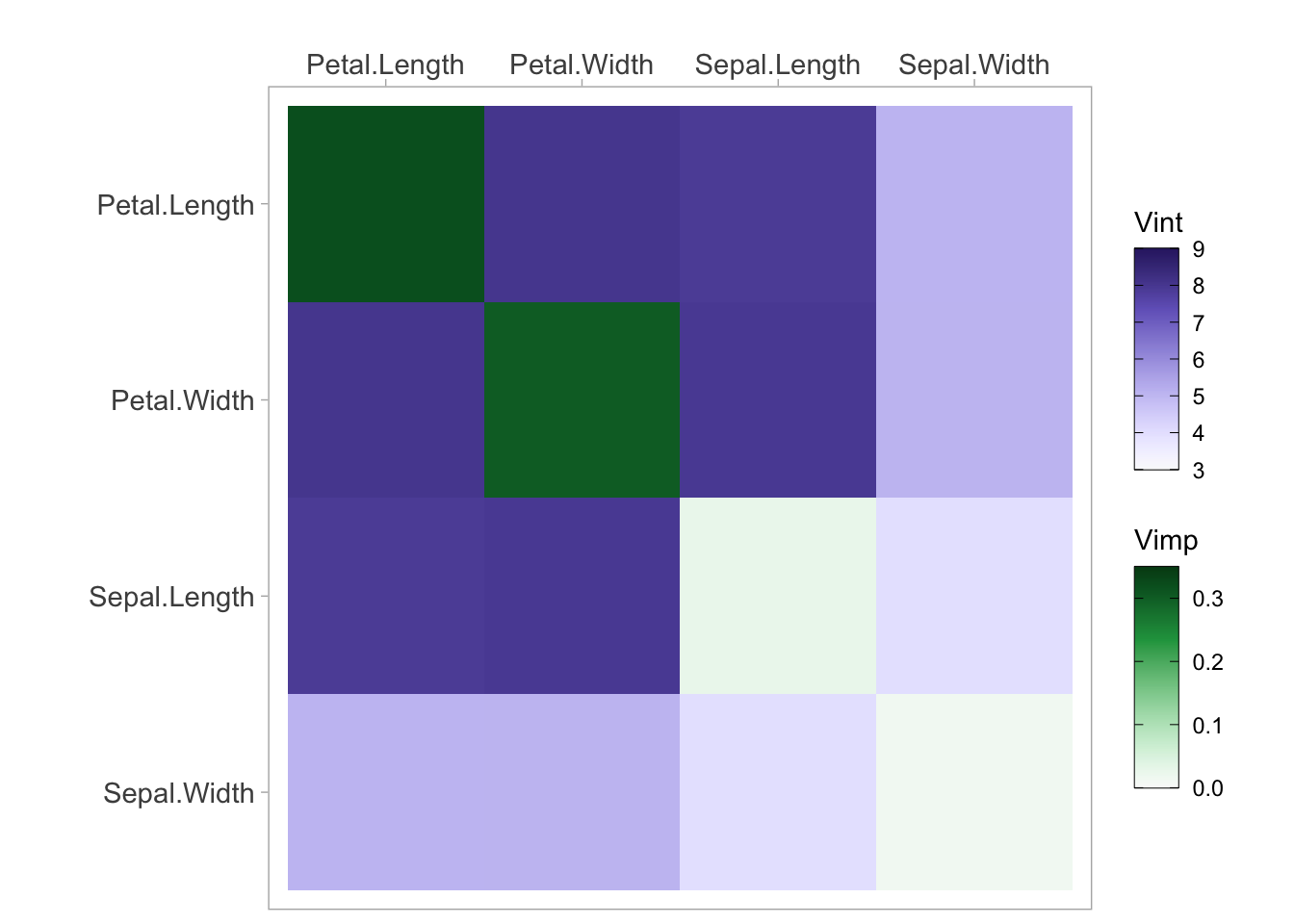

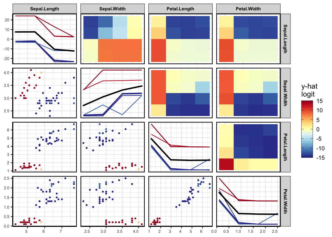
Figure 3: Heatmap of a ranger random forest classification fit displaying 2-way interaction strength on the off diagonal and individual variable importance on the diagonal.

PDP

pdpPairs(data = iris, 
         fit =  rf, 
         response = "Species", 
         nmax = 50, 
         gridSize = 4,         
         nIce = 10,
         class = 'setosa')

Figure 4: Generalized pairs partial dependence plot for a ranger random forest classification fit.