bartMan
bartManVignette.RmdIntroduction
![]()
For more detailed information and a comprehensive discussion, please
refer to our paper associated with this document, available at DOI: 10.52933/jdssv.v4i1.79.
Tree-based regression and classification has become a standard tool in
modern data science. Bayesian Additive Regression Trees (BART)1 has in
particular gained wide popularity due its flexibility in dealing with
interactions and non-linear effects. BART is a Bayesian tree-based
machine learning method that can be applied to both regression and
classification problems and yields competitive or superior results when
compared to other predictive models. As a Bayesian model, BART allows
the practitioner to explore the uncertainty around predictions through
the posterior distribution. In the bartMan package, we
present new visualisation techniques for exploring BART models. We
construct conventional plots to analyze a model’s performance and
stability as well as create new tree-based plots to analyze variable
importance, interaction, and tree structure. We employ Value Suppressing
Uncertainty Palettes (VSUP)2 to construct heatmaps that display variable
importance and interactions jointly using color scale to represent
posterior uncertainty. Our new visualisations are designed to work with
the most popular BART R packages available, namely BART3,
dbarts4, and bartMachine5.
In this document, we demonstrate our visualisations for evaluation of
BART models using the bartMan (BART Model ANalysis)
package.
Background
BART (Bayesian Additive Regression Trees) is a Bayesian non-parametric model using an ensemble of trees for predicting continuous and multi-class responses. Unlike linear regression, BART adapts a flexible functional form, uncovering main and interaction effects. The model is formulated as
\[ y_i = \sum_{j=1}^m g(x_i, T_j, M_j) + \varepsilon_i \]
with \(\varepsilon_i \sim N(0, \sigma^2)\), where \(g(x_i, T_j, M_j) = \mu_{j\ell}\) maps observations to predicted values in the terminal node \(\ell\) of tree \(j\). \(T_j\) and \(M_j\) denote the tree’s structure and the set of predicted values at its terminal nodes, respectively. Tree structures involve binary splits \([x_j \leq c]\), with variables and splits randomly chosen and updated through the model fitting process. This updating occurs via Markov chain Monte Carlo methods, involving tree modifications like growing, pruning, changing, or swapping nodes, with specifics depending on the implementation.
Inclusion Variable Importance
Chipman et al. (2010) propose a method called the inclusion proportion to evaluate the variable importance in a BART (Bayesian Additive Regression Trees) model from the posterior samples of the tree structures. This measure of variable importance first calculates for each iteration the proportion of times a variable is used to split nodes considering all \(m\) trees, and then averages these proportions across all iterations.
More formally, let \(K\) be the number of posterior samples obtained from a BART model. Let \(c_{rk}\) be the number of splitting rules using the \(r\)th predictor as a split variable in the \(k\)th posterior sample of the trees’ structure across \(m\) trees. Additionally, let \(c_{.k} = \sum_{r=1}^p c_{rk}\) represent the total number of splitting rules found in the \(k\)th posterior sample across the total \(p\) variables. Therefore, \(z_{rk} = \frac{c_{rk}}{c_{.k}}\) is the proportion of splitting rules for the \(r\)th variable, and the average use per splitting rule is given by:
\[ \text{VImp}_{\text{r}} = \frac{1}{K} \sum_{k=1}^K z_{rk} \]
Inclusion Variable Interactions
Variable interaction refers to the combined effect of two or more variables on the response. We focus on bivariate interactions, identifying them through the dependency of tree structures on multiple variables. Chipman et al. (2010)6 and Kapelner & Bleich (2016)7 introduced interaction measures based on the analysis of successive splitting rules in tree models. Similar approaches are applied in random forests, using minimal depth to evaluate interaction and importance. In contrast to random forests, where splits are optimized, BART models employ a stochastic search, treating the order of splits as inconsequential. The interaction strength between two variables \(r\) and \(q\) is quantified by
\[ \text{VInt}_{\text{rq}} = \frac{1}{K} \sum_{k=1}^K z_{rqk} \]
Install instructions
To install the development version from GitHub, use:
# install.packages("devtools")
#devtools::install_github("AlanInglis/bartMan")
library(bartMan)
bartMan
The data used in the following examples is simulated from the Friedman benchmark problem 78. This benchmark problem is commonly used for testing purposes. The output is created according to the equation:
## Create Friedman data
fData  <- function(n = 200, sigma = 1.0, seed = 1701, nvar = 5) {
  set.seed(seed)
  x <- matrix(runif(n * nvar), n, nvar)
  colnames(x) <- paste0("x", 1:nvar)

  Ey <- 10 * sin(pi * x[, 1] * x[, 2]) + 20 * (x[, 3] - 0.5)^2 + 10 * x[, 4] + 5 * x[, 5]
  y <- rnorm(n, Ey, sigma)

  data <- as.data.frame(cbind(x, y))
  return(data)
}

f_data <- fData(nvar = 10)
x <- f_data[, 1:10]
y <- f_data$y
Now we will create a basic BART model using the dbarts
package. However, the visualisation process outlined in this document is
identical for any of the dbarts, BART, or
bartMachine BART packages.
To begin we load the libraries and then create our models.
# create dbarts model:
set.seed(1701)
dbartModel <- bart(x,
                   y,
                   ntree = 20,
                   keeptrees = TRUE,
                   nskip = 100,
                   ndpost = 1000
)
In dbartModel we have selected there to be 20 trees,
1000 iterations, and a burn-in of 100. Once the model is built we can
extract the data concerning the trees via the
extractTreeData function.
# Create data frames ------------------------------------------------------
trees_data <- extractTreeData(model = dbartModel, data = fData)
The object created by the extractTreeData function is a
list containing five elements. These are:
- Tree Data Frame - A data frame containing tree attributes.
- Variable Name - The names of the variables used in building the model.
- nMCMC - The total number of iterations (posterior draws) after burn in.
- nTree - The total number of trees grown in the sum-of-trees model.
- nVar - The total number of covariates used in the model.
The tree data frame created from the extractTreeData
function contains 17 columns concerning different attributes associated
with the trees, and the structure of which is the same across all BART
packages. It can be accessed via $structure. This data
frame is used by many of the bartMan functions to create
the visualisations shown later. In the code below, we take a look at the
structure of the data frame of trees.
options(tibble.width = Inf) # used to display full tibble in output
head(trees_data$structure, 5)
#> # A tibble: 5 × 17
#>   var   splitValue terminal leafValue iteration treeNum  node childLeft
#>   <chr>      <dbl> <lgl>        <dbl>     <int>   <int> <int>     <int>
#> 1 x2         0.893 FALSE      NA              1       1     1         2
#> 2 x1         0.564 FALSE      NA              1       1     2         3
#> 3 x8         0.515 FALSE      NA              1       1     3         4
#> 4 <NA>      NA     TRUE       -0.0403         1       1     4        NA
#> 5 <NA>      NA     TRUE       -0.0381         1       1     5        NA
#>   childRight parent depth depthMax isStump label         value obsNode     noObs
#>        <int>  <int> <dbl>    <dbl> <lgl>   <chr>         <dbl> <list>      <int>
#> 1          7     NA     0        4 FALSE   x2  ≤  0.89  0.893  <dbl [200]>   200
#> 2          6      1     1        4 FALSE   x1  ≤  0.56  0.564  <dbl [171]>   171
#> 3          5      2     2        4 FALSE   x8  ≤  0.51  0.515  <dbl [95]>     95
#> 4         NA      3     3        4 FALSE   -0.04       -0.0403 <dbl [57]>     57
#> 5         NA      3     3        4 FALSE   -0.04       -0.0381 <dbl [38]>     38
In the following table, each of the columns of
trees_data$structure are explained:
| Column | Description |
|---|---|
| var | Variable name used for splitting. |
| splitValue | Value of the variable at which the split occurs. |
| terminal | Logical indicator if the node is terminal (TRUE) or not (FALSE). |
| leafValue | Value at the leaf node, NA for non-terminal nodes. |
| iteration | Iteration number. |
| treeNum | Tree number. |
| node | Unique identifier for the node (following depth-first-left-side traversal). |
| childLeft | Identifier for the left child of the node, NA for terminal nodes. |
| childRight | Identifier for the right child of the node, NA for terminal nodes. |
| parent | Identifier for the parent of the node, NA for root nodes. |
| depth | Depth of the node in the tree, starting from 0 for root nodes. |
| depthMax | Maximum depth of the tree. |
| isStump | Logical indicator if the node is a stump (TRUE) or not (FALSE). |
| label | Node label. |
| value | The value in a node (i.e., either the split value or leaf value). |
| obsNode | List of observations in the node, represented in a compact form. |
| noObs | Number of observations in the node. |
The trees in the data frame are ordered in a depth-first left-side
traversal method. An example of this is shown below in Figure 1. Here we
can see the ordering and node number used in this method. For clarity,
the $structure$var column (created from the
extractTreeData() function) would be ordered as
X1, NA, X2, X2, NA, NA, NA, where NA
indicates terminal (or leaf) nodes.

Visualisations
VIVI-VSUP
In Inglis et al. (2022)9, the authors propose using a heatmap to display both variable importance (VImp) and variable interactions (VInt) simultaneously (together VIVI), where the importance values are on the diagonal and interaction values on the off-diagonal. We adapt the heatmap displays of importance and interactions to include the uncertainty by use of a VSUP. To begin we fist generate a heatmap containing the raw VIVI values without uncertainty.
stdMat <- viviBartMatrix(trees_data,
                          type = 'standard',
                          metric = 'propMean')
Now we create a list of two matrices. One containing the raw
inclusion proportions and one containing the uncertainties. Here we use
the coefficient of variation as our uncertainty measure. However the
standard deviation or standard error is also available by setting
metricError = 'SD' or metricError = 'SE', in
the code below.
vsupMat <- viviBartMatrix(trees_data,
                          type = 'vsup',
                          metric = 'propMean',
                          metricError = "CV")
Once the matrices have been created, they can be plotted displaying a VSUP plot with the uncertainty included. For illustration purposes, we show the plot without uncertainty in Figure 1 and with uncertainty in Figure 2:
viviBartPlot(stdMat)
viviBartPlot(vsupMat,
             max_desat = 1,
             pow_desat = 0.6,
             max_light = 0.6,
             pow_light = 1,
             label = 'CV')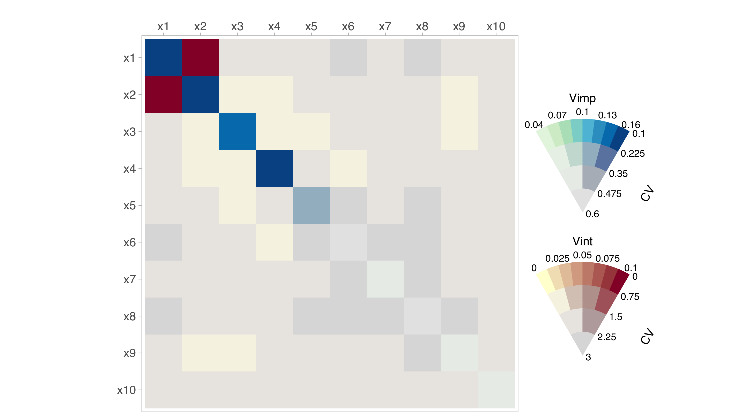
In Figure 3, when we include uncertainty, both the importance and interaction values for the noise variables have a high coefficient of variation associated with them and as such, the most influential variables are highlighted.
When plotting the VSUP with uncertainty, some of the relevant function arguments include:
-
unc_levels: The number of uncertainty levels -
max_desat: The maximum desaturation level of the uncertainty palette -
pow_desat: The power of desaturation level -
max_light: The maximum light brightness of the uncertainty palette -
pow_light: The power of light level
Tree Based Plots
Here we examine more closely the structure of the decision trees created when building a BART model. Examining the tree structure may yield information on the stability and variability of the tree structures as the algorithm iterates to create the posterior. By sorting and colouring the trees appropriately we can identify important variables and common interactions between variables for a given iteration. Alternatively we can look at how a single tree evolves through the iteration to explore the fitting algorithm’s stability.
To plot an individual tree, we can choose to display it either in dendrogram format, or icicle format. Additionally, we can choose which tree number or iteration to display:
plotSingleTree(trees = trees_data, treeNo = 1, iter = 1, plotType = "dendrogram")
plotSingleTree(trees = trees_data, treeNo = 1, iter = 1, plotType = "icicle")
The plotTrees function allows for a few different
options when plotting. The function arguments for plotTrees
are outlined as follows:
• trees: A data frame of trees, usually created via
extractTreeData().
• iter: An integer specifying the iteration number of
trees to be included in the output. If NULL, trees from all iterations
are included.
• treeNo: An integer specifying the number of the tree
to include in the output. If NULL, all trees are included.
• fillBy: A character string specifying the attribute to
color nodes by. Options are ‘response’ for coloring nodes based on their
mean response values or ‘mu’ for coloring nodes based on their predicted
value, or NULL for no specific fill attribute.
• sizeNodes A logical value indicating whether to adjust
node sizes. If TRUE, node sizes are adjusted; if FALSE, all nodes are
given the same size.
• removeStump A logical value. If TRUE, then stumps are
removed from plot.
• selectedVars A vector of selected variables to
display. Either a character vector of names or the variables column
number.
• pal A colour palette for node colouring. Palette is
used when ‘fillBy’ is specified for gradient colouring.
• center_Mu A logical value indicating whether to center
the color scale for the ‘mu’ attribute around zero. Applicable only when
‘fillBy’ is set to “mu”.
• cluster A character string that specifies the
criterion for reordering trees in the output. Currently supports “depth”
for ordering by the maximum depth of nodes, and “var” for a clustering
based on variables. If NULL, no reordering is performed.
For example, we can chose to display all the trees from a selected iteration:
plotTrees(trees = trees_data, iter = 1)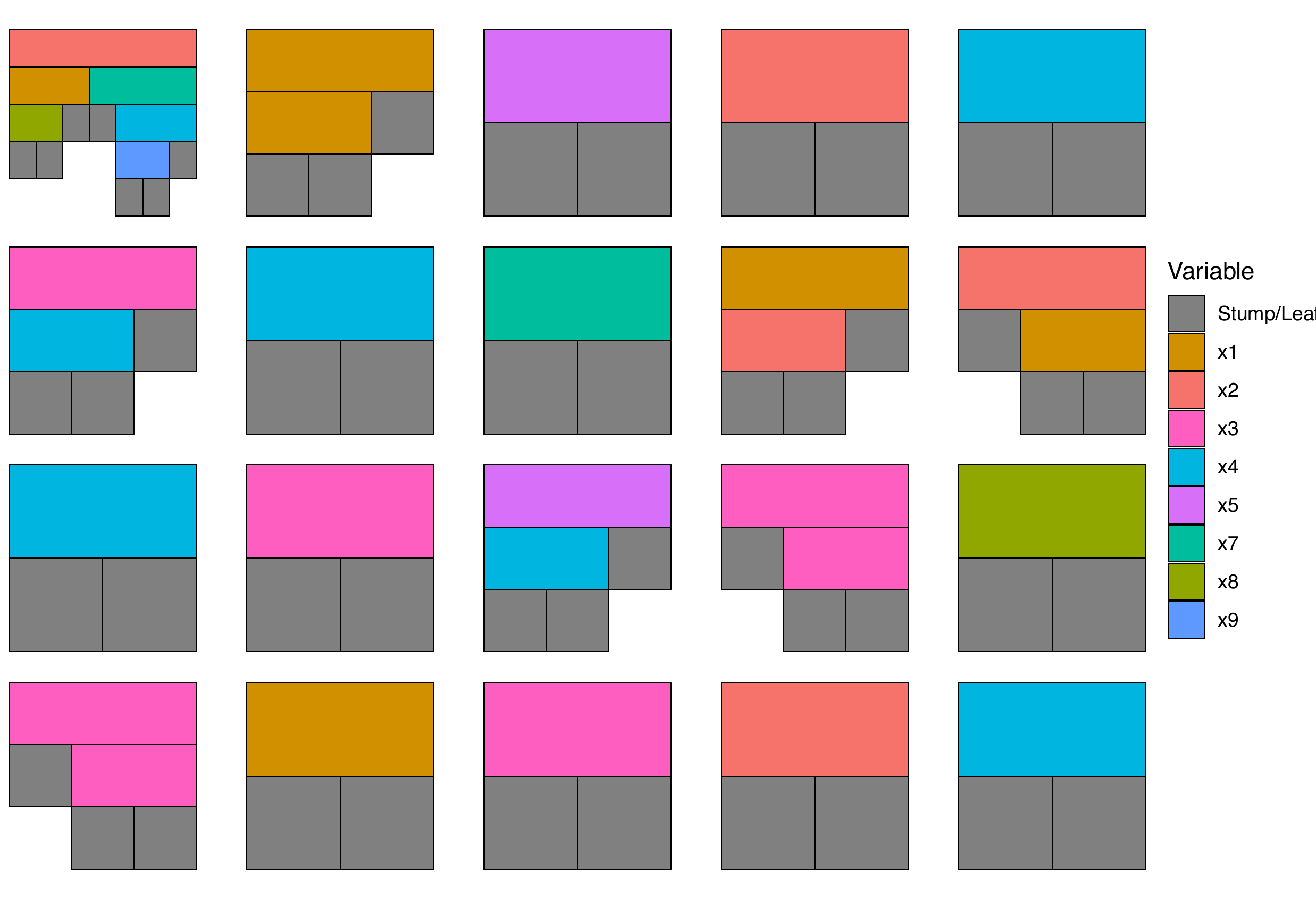
When the number of variables or trees is large it can become hard to
identify interesting features. By using the selectedVars
argument, we can highlight selected variables by colouring them brightly
while uniformly colouring the remaining variables a light grey.

We can plot a single tree over all iterations by selecting a tree via
the treeNo argument. This shows us visually BART’s
grow, prune, change, swap mechanisms in action.
plotTrees(trees = trees_data, treeNo = 1)
When viewing the trees, it can be useful to view different aspects or metrics. In Figure 7 we show some of these aspects by displaying all the trees in a selected iteration. For example, in (a) we color them by the terminal node parameter value. In (b) we color terminal nodes and stumps by the mean response. In (c) we sort the trees by structure starting with the most common tree structure and descending to the least common tree found (useful for identifying the most important splits). Finally, in (d) we sort the trees by depth. As the \(\mu\) values in (a) are centered around zero by default, we use a single-hue, colorblind friendly, diverging color palette to display the values. For comparison, we use the same palette to represent the mean response values in (b).
plotTrees(trees = trees_data, iter = 1, sizeNode = T, fillBy = 'mu')
plotTrees(trees = trees_data, iter = 1, sizeNode = T, fillBy = 'response')
plotTrees(trees = trees_data, iter = 1, cluster = "var")
plotTrees(trees = trees_data, iter = 1, cluster = "depth")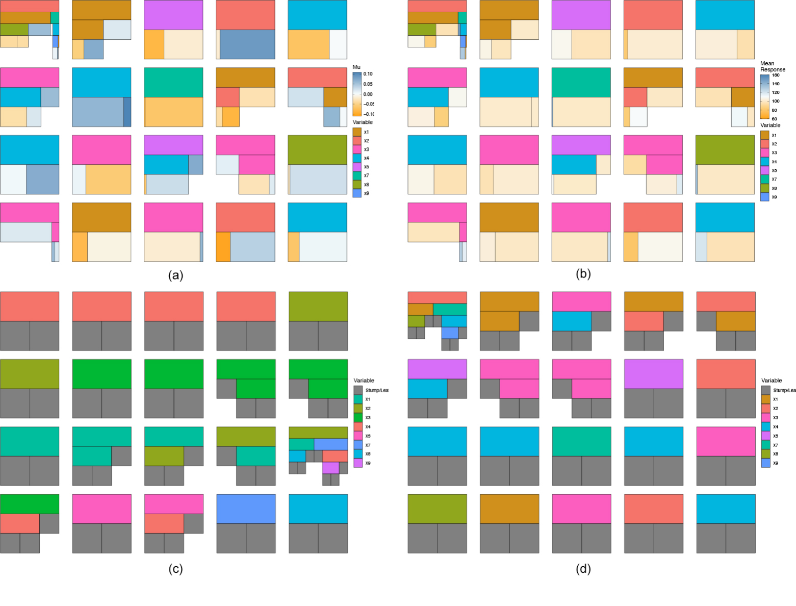
As an alternative to the sorting of the tree structures, seen in
Figure 8 (c), we provide a bar plot summarizing the tree structures.
Here we choose to display the top 10 most frequent tree structures,
however displaying a single tree across iterations is possible via the
iter argument.
treeBarPlot(trees = trees_data, topTrees = 10, iter = NULL)
An interesting finding from looking at Figure 9 is we can see that the most frequent tree is a tree with a single binary split on \(x_3\). However, looking at the rest of the trees, we can see the prevalence of splits on \(x_1\) and \(x_2\), indicating that these are important variables.
Proximity Matrix and Multidimensional Scaling
Proximity matrices combined with multidimensional scaling (MDS) are commonly used in random forests to identify outlying observations10. When two observations lie in the same terminal node repeatedly they can be said to be similar, and so an \(N × N\) proximity matrix is obtained by accumulating the number of times at which this occurs for each pair of observations, and subsequently divided by the total number of trees. A higher value indicates that two observations are more similar.
To begin, we fist create a proximity matrix. This can be seriated to
group similar observations together by setting
reorder = TRUE. The normailze argument will
divide the proximity scores by the total number of trees. Additionally,
we can choose to get the proximity matrix for a single iteration (as
shown below) or over all iterations, the latter is achieved by setting
iter = NUll.
bmProx <- proximityMatrix(trees = trees_data,
                          reorder = TRUE,
                          normalize = TRUE,
                          iter = 1)
We can then visualize the proximity matrix using the
plotProximity function.
plotProximity(matrix = bmProx) +
  theme(axis.text.x = element_text(angle = 90,))
The proximity matrix can then be visualized using classical MDS (henceforth MDS) to plot their relationship in a lower dimensional projection.
In BART, as there is a proximity matrix for every iteration and a
posterior distribution of proximity matrices. We introduce a rotational
constraint so that we can similarly obtain a posterior distribution of
each observation in the lower dimensional space. We first choose a
target iteration (as shown above) and apply MDS. For each subsequent
iteration we rotate the MDS solution matrix to match this target as
closely as possible using Procrustes’ method. We end up with a point for
each observation per iteration per MDS dimension.We then group the
observations by the mean of each group and produce a scatter plot, where
each point represents the centroid of the location of each observation
across all the MDS solutions. We extend this further by displaying
confidence ellipses around each observation’s posterior location in the
reduced space (via the level argument). Since these are
often overlapping we have created an interactive version that highlights
an observation’s ellipse and displays the observation number when
hovering the mouse pointer above the ellipse (Figure 11 shows a
screenshot of this interaction in use). However, non-interactive
versions are available via the plotType argument.
mdsBart(trees = trees_data, data = f_data, target =  bmProx,
plotType = 'interactive', level = 0.25, response = 'y') 
Enhanced BART model diagnostics
In addition to the above, we also provide visualisations for general
diagnostics of a BART model. These include checking for convergence, the
stability of the trees, the efficiency of the algorithm, and the
predictive performance of the model. To begin we take a look at some
general diagnostics to assess the stability of the model fit. The
burnIn argument should be set to the burn-in value selected
when building the model and indicates the separation between the pre and
post burn-in period in the plot.
bartDiag(model = dbartModel, response = f_data$y, burnIn = 100, data = fData)
Acceptance Rate
The post burn-in percentage acceptance rate across all iterations can also be visualized, where each point represents a single iteration. A regression line is shown to indicate the changes in acceptance rate across iterations and to identify the mean rate.
acceptRate(trees = trees_data)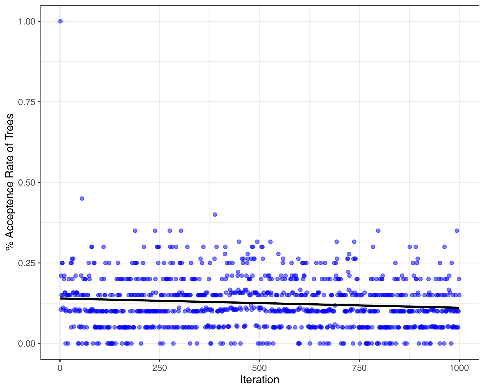
Mean Tree Depth and Mean Tree Nodes
As with the acceptance rate, the average tree depth and average number of all nodes per iteration can give an insight into the fit’s stability. Figure 11 displays these two metrics. A locally estimated scatter plot smoothing (LOESS) regression line is shown to indicate the changes in both the average tree depth and the average number of nodes across iterations:

Split Densities
Figure 12 shows the densities of split values over all post burn-in iterations for each variable for both models (in green), combined with the densities of the predictor variables (labeled “data”, in red):
splitDensity(trees = trees_data, data = f_data, display = 'dataSplit')
Alternatively, we can just examine the plit value densities in a ridge plot style.
splitDensity(trees = trees_data, data = f_data, display = 'ridges')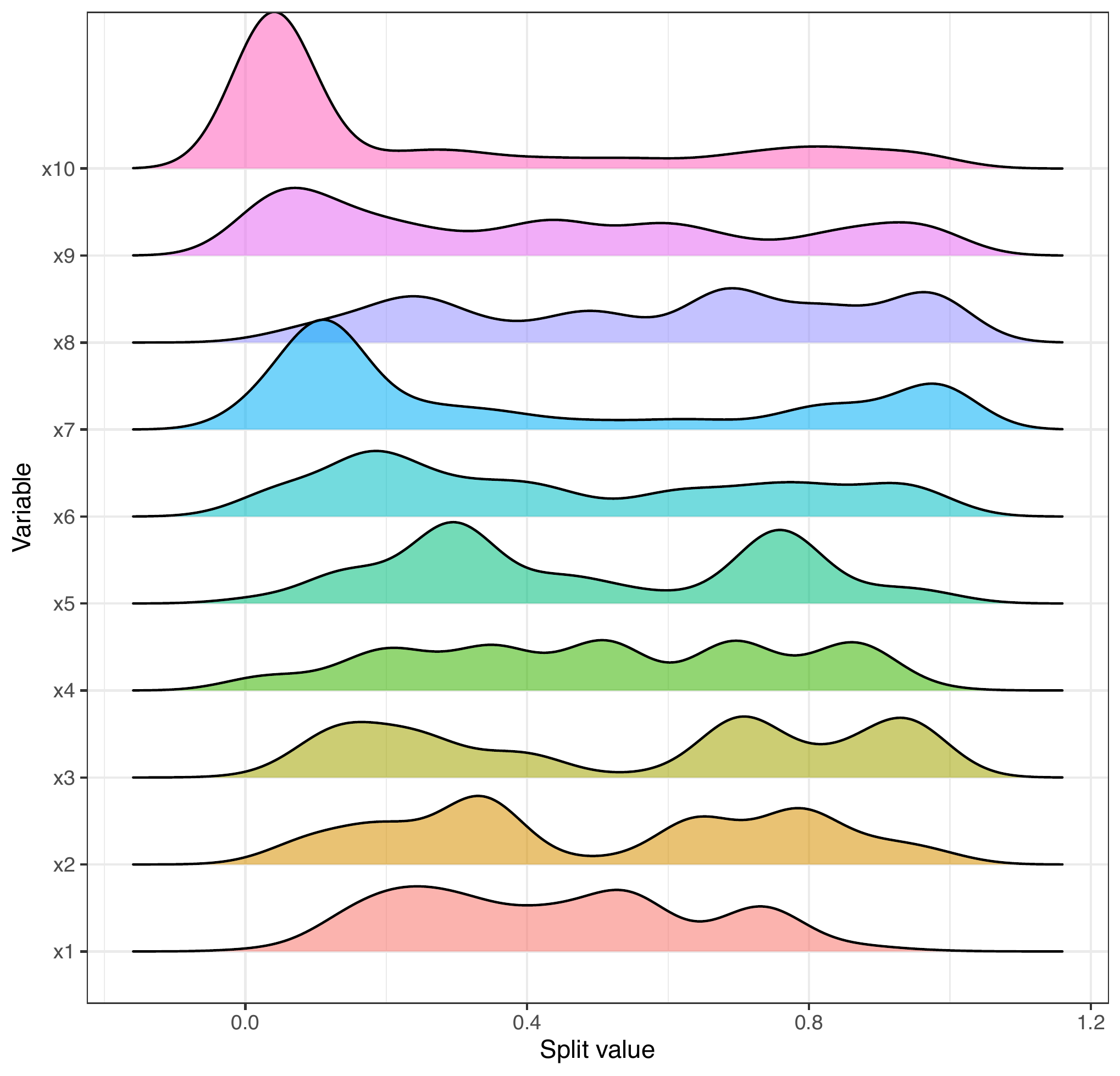
Additional Importance and Interaction plots.
To assess inclusion proportions related to variable importance and
interactions, we offer functions that facilitate the extraction and
visualisation of these metrics. For instance, the viviBart
function allows retrieval of a list encompassing both variable
importance and interactions, along with their associated error metrics,
an example of which is shown below. To select either just the importance
or just the interactions, the out argument should be set to
'vimp' or 'vint', respectively.
# show both vimp and vint
viviBart(trees = trees_data, out = 'vivi')
#> $Vimp
#>     variable count   propMean         SD        CV           SE    lowerCI
#> x1        x1  7966 0.22571216 0.03254446 0.1441857 0.0010291463 0.22369504
#> x2        x2  6366 0.18049674 0.03495082 0.1936368 0.0011052419 0.17833047
#> x3        x3  5898 0.16736770 0.03651604 0.2181786 0.0011547387 0.16510441
#> x4        x4  5645 0.16047108 0.03099483 0.1931490 0.0009801426 0.15855000
#> x5        x5  4094 0.11537889 0.03484564 0.3020105 0.0011019159 0.11321914
#> x6        x6   619 0.01743208 0.02085356 1.1962747 0.0006594474 0.01613957
#> x7        x7  1244 0.03477908 0.02367593 0.6807519 0.0007486986 0.03331163
#> x8        x8  1691 0.04786435 0.03205731 0.6697534 0.0010137411 0.04587742
#> x9        x9   682 0.01926840 0.02344669 1.2168473 0.0007414496 0.01781515
#> x10      x10  1119 0.03122951 0.03109255 0.9956142 0.0009832327 0.02930238
#>        upperCI     lowerQ     median     upperQ
#> x1  0.22772929 0.20000000 0.22222222 0.25000000
#> x2  0.18266302 0.15625000 0.17948718 0.20000000
#> x3  0.16963099 0.13888889 0.17073171 0.19444444
#> x4  0.16239216 0.13888889 0.15625000 0.18181818
#> x5  0.11753865 0.08823529 0.11111111 0.13513514
#> x6  0.01872460 0.00000000 0.00000000 0.02857143
#> x7  0.03624653 0.02631579 0.02941176 0.05405405
#> x8  0.04985128 0.02777778 0.03225806 0.06250000
#> x9  0.02072164 0.00000000 0.00000000 0.02941176
#> x10 0.03315665 0.00000000 0.02777778 0.05555556
#>
#> $Vint
#> # A tibble: 55 × 10
#>    var    count propMean      SD    CV       SE lowerQ median upperQ adjusted
#>    <chr>  <dbl>    <dbl>   <dbl> <dbl>    <dbl>  <dbl>  <dbl>  <dbl>    <dbl>
#>  1 x1:x1  1.96   0.0728  0.0282  0.388 0.000893 0.0588 0.0694 0.0833   0.0969
#>  2 x1:x2  2.75   0.101   0.0343  0.339 0.00108  0.0741 0.0938 0.12     0.299
#>  3 x1:x3  0.843  0.0291  0.0263  0.904 0.000833 0      0.0345 0.0435   0
#>  4 x1:x4  0.136  0.00463 0.0134  2.89  0.000423 0      0      0        0
#>  5 x1:x5  1.20   0.0424  0.0419  0.988 0.00133  0      0.0357 0.0741   0.102
#>  6 x1:x6  0.09   0.00328 0.0111  3.37  0.000350 0      0      0        0
#>  7 x1:x7  0.058  0.00215 0.00887 4.13  0.000281 0      0      0        0
#>  8 x1:x8  0.334  0.0124  0.0216  1.74  0.000683 0      0      0.0296   0.0156
#>  9 x1:x9  0.136  0.00523 0.0148  2.83  0.000468 0      0      0        0.0133
#> 10 x1:x10 0.105  0.00381 0.0124  3.25  0.000392 0      0      0        0
#> # ℹ 45 more rows
To visualize the inclusion proportion variable importance (with their
25% to 75% quantile interval included) we use the vimpPlot
function.
# plot inclusion proportions of each variable:
vimpPlot(trees = trees_data, plotType = 'point')
vimpPlot(trees = trees_data, plotType = 'barplot')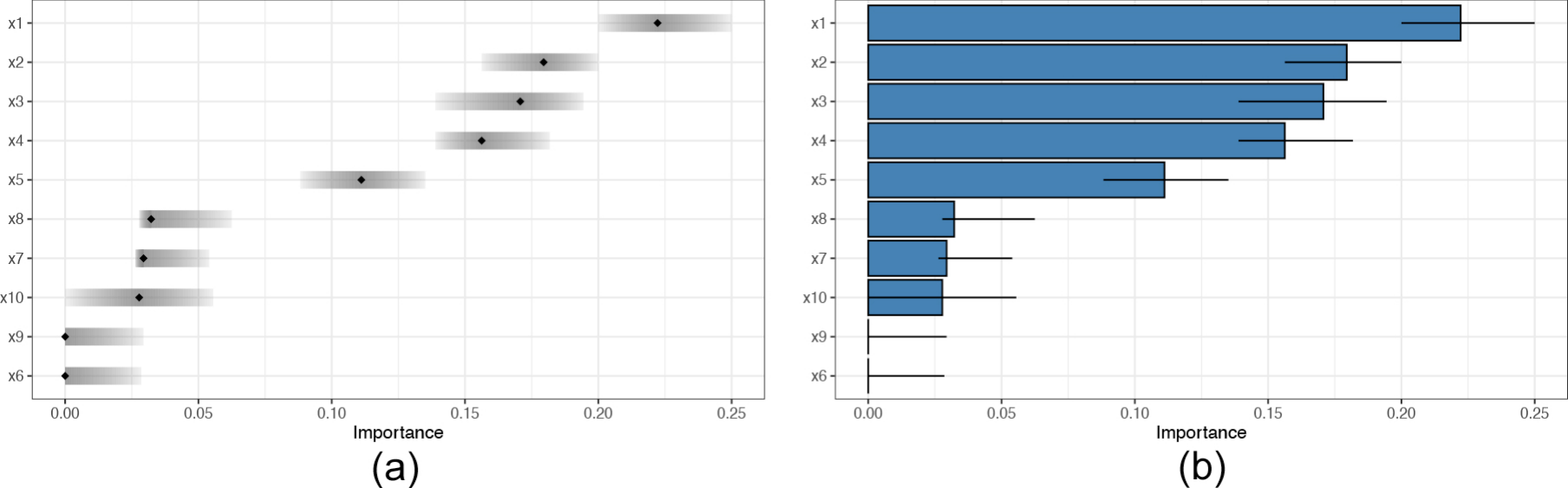
An alternative method to display the inclusion proportions is by
using a Letter-value plot11. This type of plot is useful for
visualizing the distribution of a continuous variable (here variable
inclusion proportions), with the inner-most box showing the lower and
upper fourths, as with a conventional box plot, the median value being
shown as a black line and outliers as blue triangles. Each extending
section is drawn at incremental steps of upper and lower eights,
sixteenths and so on until a stopping rule has been reached. The color
of each box corresponds to the density of the data with darker shades
indicating higher data density. Note, when
plotType = 'lvp', the geom_lv function from
the lvplot package is used. This function requires the
ggplot2 package to be loaded.
library("ggplot2")
vimpPlot(trees = trees_data, plotType = 'lvp') + coord_flip()
Similarly, we provide a function for viewing the inclusion proportions for interactions, again with 25% to 75% quantile interval included. In Figure 19, we display only the top 5 strongest variable pair interactions.
# plot inclusion proportions of each variable pair:
vintPlot(trees = trees_data, top = 5)
Null model inclusion proportions
In our package we also implement one of the variable selection procedures developed in Bleich et al. (2014)12, specifically, the so-called local threshold procedure. In this method, the proportion of splitting rules is calculated, then the response variable is randomly permuted, which has the effect of breaking the relationship between the response and the covariates. The model is then re-built as a null model using the permuted response. From this, the null proportion, is calculated and a new measure of importance is obtained.
When using this method, there are three key arguments:
numRep, numTreesRep, and alpha.
numRep determines the number of replicates to perform for
the BART null model’s variable inclusion proportions. Whereas,
numTreesRep determines the number of trees to be used in
the replicates. alpha sets the cut-off level for the
thresholds. That is, a predictor is deemed important if its variable
inclusion proportion exceeds the 1 − \(\alpha\) quantile of its own null
distribution. If setting shift = TRUE, the inclusion
proportions are shifted by the difference in distance between the
quantile and the value of the inclusion proportion point.
localProcedure(model = dbartModel,
               data = f_data,
               numRep = 5,
               numTreesRep = 5,
               alpha = 0.5,
               shift = FALSE)
shift = FALSE, whereas in the right plot,
shift = TRUE.
Single Permutation Null Model
We also provide the functionality for a variable selection approach which creates a null model by permuting the response once, rebuilding the model, and calculating the inclusion proportion on the null model. The final result displayed is the original model’s inclusion proportion minus the null inclusion proportion. This function is available for both the importance and the interactions.
permVimp(model = dbartModel, data = f_data, response = 'y',  numTreesPerm = 5)
permVimp(model = dbartModel, data = f_data, response = 'y',  numTreesPerm = 10)
permVimp(model = dbartModel, data = f_data, response = 'y',  numTreesPerm = 20)
numTreesPerm is equal to 5, 10, and 20.
In Figure 21, we compare the difference in importance when
numTreesPerm is equal to 5, 10, and 20. We can see that as
we increase the number of trees to be used in the replicates, variable
\(\x_1\) and \(\x_2\) start to emerge as the most
important variables.
For assessing the interactions using the single permutation method we have:
permVint(trees = trees_data,model = dbartModel, data = f_data, response = 'y', top = 5)
Combining Categorical Variables
If any of the variables used to build the BART model are categorical, the aforementioned BART packages replace the categorical variables with \(d\) dummy variables, where \(d\) is the number of factor levels. However, we provide the functionality to adjust the inclusion proportions for variable importance and interaction by aggregating over factor levels. This provides a complete picture of the importance of a factor, rather than that associated with individual factor levels.
In the following example, we build a BART model using the
BART package where one of the covariates is a factor and
extract the tree data.
library(BART)
#> Loading required package: nlme
#> Loading required package: nnet
#> Loading required package: survival

data(iris)
set.seed(1701)
bartModel <- wbart(x.train = iris[,2:5],
                   y.train = iris[,1],
                   nskip = 10,
                   ndpost = 100,
                   nkeeptreedraws = 100,
                   ntree = 5
)

bt_trees <- extractTreeData(model = bartModel, data = iris)
As Species is a factor with three levels, it is split
into three dummy variables when building the model. For a practical
example of what this looks like, we examine the variable importance
inclusion proportions both before and after aggregating over the factor
levels.
# extract the vimp data
vimpData <- viviBart(trees = bt_trees,  out = 'vimp')
vimpData[,1:3] # looking at the relevant columns
#>                  variable count   propMean
#> Sepal.Width   Sepal.Width   234 0.23382715
#> Petal.Length Petal.Length   416 0.40474595
#> Petal.Width   Petal.Width   181 0.19423754
#> Species1         Species1    95 0.09627939
#> Species2         Species2    32 0.02590565
#> Species3         Species3    38 0.04500433
To combine the dummy factor variables, we use the
combineDummy() function. This function takes in a tree data
created by extractTreeData(), combines the dummy factors,
and outputs a new tree data object with the combined dummies.
bt_trees_combined <- combineDummy(trees = bt_trees)Looking again we see the dummies are combined:
# extract the vimp data
vimpData_combined <- viviBart(trees = bt_trees_combined,  out = 'vimp')
vimpData_combined[,1:3] # looking at the relevant columns
#>                  variable count  propMean
#> Sepal.Length Sepal.Length     0 0.0000000
#> Sepal.Width   Sepal.Width   234 0.2338271
#> Petal.Length Petal.Length   416 0.4047459
#> Petal.Width   Petal.Width   181 0.1942375
#> Species           Species   165 0.1671894
Taking a look at the trees before and after combining the dummy variables

Creating Your Own Data Frame Of Trees To Plot
The bartMan package, initially designed for three
primary BART packages, also allows users to input their own data to
create an object comparable with the extractTreeData()
function output. This integration is facilitated through the
tree_dataframe() function, which ensures its output aligns
with extractTreeData(). The tree_dataframe()
function requires the original dataset used to build the model and a
tree data frame. The tree data frame must include a var
column that follows a depth-first left-side traversal order, a
value column with the split or terminal node values, and
columns for iteration and treeNum to denote
the specific iteration and tree number, respectively.
In the example below, we have both a data set f_data and
a tree data frame df_tree containing the needed
columns.
# Original Data
f_data <- data.frame(
  x1 = c(0.127393428, 0.766723202, 0.054421675, 0.561384595, 0.937597936,
         0.296445079, 0.665117463, 0.652215607, 0.002313313, 0.661490602),
  x2 = c(0.85600486, 0.02407293, 0.51942589, 0.20590965, 0.71206404,
         0.27272126, 0.66765977, 0.94837341, 0.46710461, 0.84157353),
  x3 = c(0.4791849, 0.8265008, 0.1076198, 0.2213454, 0.6717478,
         0.5053170, 0.8849426, 0.3560469, 0.5732139, 0.5091688),
  x4 = c(0.55089910, 0.35612092, 0.80230714, 0.73043828, 0.72341749,
         0.98789408, 0.04751297, 0.06630861, 0.55040341, 0.95719901),
  x5 = c(0.9201376, 0.9279873, 0.5993939, 0.1135139, 0.2472984,
         0.4514940, 0.3097986, 0.2608917, 0.5375610, 0.9608329),
  y = c(14.318655, 12.052513, 13.689970, 13.433919, 18.542184,
        14.927344, 14.843248, 13.611167, 7.777591, 23.895456)
  )


# Your own data frame of trees
df_tree <- data.frame(
  var = c("x3", "x1", NA, NA, NA, "x1", NA, NA, "x3", NA, NA, "x1", NA, NA),
  value = c(0.823,0.771,-0.0433,0.0188,-0.252,0.215,-0.269,0.117,0.823,0.0036,-0.244,0.215,-0.222,0.0783),
  iteration = c(1, 1, 1, 1, 1, 1, 1, 1, 2, 2, 2, 2, 2, 2),
  treeNum = c(1, 1, 1, 1, 1, 2, 2, 2, 1, 1, 1, 2, 2, 2)
)

# take a look at the dataframe of trees
df_tree
#>     var   value iteration treeNum
#> 1    x3  0.8230         1       1
#> 2    x1  0.7710         1       1
#> 3  <NA> -0.0433         1       1
#> 4  <NA>  0.0188         1       1
#> 5  <NA> -0.2520         1       1
#> 6    x1  0.2150         1       2
#> 7  <NA> -0.2690         1       2
#> 8  <NA>  0.1170         1       2
#> 9    x3  0.8230         2       1
#> 10 <NA>  0.0036         2       1
#> 11 <NA> -0.2440         2       1
#> 12   x1  0.2150         2       2
#> 13 <NA> -0.2220         2       2
#> 14 <NA>  0.0783         2       2
Applying the tree_dataframe() function creates an object
that aligns with the output of extractTreeData(). The
response argument is an optional character argument of the
name of the response variable in your BART model. Including the response
will remove it from the list elements Variable names and
nVar.
trees_data <- tree_dataframe(data = f_data , trees = df_tree, response = 'y')
# look at tree data object
trees_data
#> Tree dataframe:
#> # A tibble: 14 × 17
#>    var   splitValue terminal leafValue iteration treeNum  node childLeft
#>    <chr>      <dbl> <lgl>        <dbl>     <dbl>   <dbl> <int>     <int>
#>  1 x3         0.823 FALSE      NA              1       1     1         2
#>  2 x1         0.771 FALSE      NA              1       1     2         3
#>  3 <NA>      NA     TRUE       -0.0433         1       1     3        NA
#>  4 <NA>      NA     TRUE        0.0188         1       1     4        NA
#>  5 <NA>      NA     TRUE       -0.252          1       1     5        NA
#>  6 x1         0.215 FALSE      NA              1       2     1         2
#>  7 <NA>      NA     TRUE       -0.269          1       2     2        NA
#>  8 <NA>      NA     TRUE        0.117          1       2     3        NA
#>  9 x3         0.823 FALSE      NA              2       1     1         2
#> 10 <NA>      NA     TRUE        0.0036         2       1     2        NA
#> 11 <NA>      NA     TRUE       -0.244          2       1     3        NA
#> 12 x1         0.215 FALSE      NA              2       2     1         2
#> 13 <NA>      NA     TRUE       -0.222          2       2     2        NA
#> 14 <NA>      NA     TRUE        0.0783         2       2     3        NA
#>    childRight parent depth depthMax isStump label         value obsNode    noObs
#>         <int>  <int> <dbl>    <dbl> <lgl>   <chr>         <dbl> <list>     <int>
#>  1          5     NA     0        2 FALSE   x3  ≤  0.82  0.823  <dbl [10]>    10
#>  2          4      1     1        2 FALSE   x1  ≤  0.77  0.771  <dbl [8]>      8
#>  3         NA      2     2        2 FALSE   -0.04       -0.0433 <dbl [7]>      7
#>  4         NA      2     2        2 FALSE   0.02         0.0188 <dbl [1]>      1
#>  5         NA      1     1        2 FALSE   -0.25       -0.252  <dbl [2]>      2
#>  6          3     NA     0        1 FALSE   x1  ≤  0.22  0.215  <dbl [10]>    10
#>  7         NA      1     1        1 FALSE   -0.27       -0.269  <dbl [3]>      3
#>  8         NA      1     1        1 FALSE   0.12         0.117  <dbl [7]>      7
#>  9          3     NA     0        1 FALSE   x3  ≤  0.82  0.823  <dbl [10]>    10
#> 10         NA      1     1        1 FALSE   0            0.0036 <dbl [8]>      8
#> 11         NA      1     1        1 FALSE   -0.24       -0.244  <dbl [2]>      2
#> 12          3     NA     0        1 FALSE   x1  ≤  0.22  0.215  <dbl [10]>    10
#> 13         NA      1     1        1 FALSE   -0.22       -0.222  <dbl [3]>      3
#> 14         NA      1     1        1 FALSE   0.08         0.0783 <dbl [7]>      7
#> Variable names:
#> [1] "x1" "x2" "x3" "x4" "x5"
#> nMCMC:
#> [1] 2
#> nTree:
#> [1] 2
#> nVar:
#> [1] 5
Once we have our newly created object, it can be used in any of the plotting functions, for example:
plotTrees(trees = trees_data, iter = NULL)
tree_dataframe() function.
Utility Functions
Tree List
In addition to the data frame of trees, we also provide an option for
separating the trees into a list, where each element is a
tidygraph object, containing the structure of every
individual tree. This allows a user to quickly access each tree for
custom data analysis or visualisation, with options for selection of
either a specific iteration, tree number, or both together. Each
tidygraph object includes node and edge information. For
example, if we want to create a list of the trees used in the first
iteration, we would do the following:
tree_list <- treeList(trees = trees_data, iter = 1, treeNo = NULL)
#> Iteration 1 Selected.
Examine the first tree yields:
tree_list[[1]]
#> # A tbl_graph: 5 nodes and 4 edges
#> #
#> # A rooted tree
#> #
#> # A tibble: 5 × 11
#>   var    node iteration treeNum label         value depthMax noObs respNode
#>   <chr> <int>     <dbl>   <dbl> <chr>         <dbl>    <dbl> <int>    <dbl>
#> 1 x3        1         1       1 x3  ≤  0.82  0.823         2    10     5.5
#> 2 x1        2         1       1 x1  ≤  0.77  0.771         2     8     5.75
#> 3 <NA>      3         1       1 -0.04       -0.0433        2     7     5.86
#> 4 <NA>      4         1       1 0.02         0.0188        2     1     5
#> 5 <NA>      5         1       1 -0.25       -0.252         2     2     4.5
#>   obsNode    isStump
#>   <list>     <lgl>
#> 1 <dbl [10]> FALSE
#> 2 <dbl [8]>  FALSE
#> 3 <dbl [7]>  FALSE
#> 4 <dbl [1]>  FALSE
#> 5 <dbl [2]>  FALSE
#> #
#> # A tibble: 4 × 2
#>    from    to
#>   <int> <int>
#> 1     1     2
#> 2     2     3
#> 3     2     4
#> # ℹ 1 more row
As we can see, it contains many of the same columns found in the data frame of trees. Specifically, var, node, iteration, treeNum, label, value, depthMax, noObs, respNode, obsNode, isStump, where each of the columns has the same meaning as outlined previously. The one exception is respNode, which contains the average response value over all observations found in a particular node.
Tree Dataframe Functions
The tree_dataframe() function internally utilises a set
of utility functions that are also available for direct use. These
functions are instrumental in processing and analysing tree
structures:
-
node_depth: This function calculates the depth of each node within the tree, assuming a binary tree structure. It requires the tree data frame to have aterminalcolumn that indicates whether a node is terminal. The function is typically used as follows:
depthList <- lapply(split(trees, ~treeNum + iteration),
                      function(x) cbind(x, depth = node_depth(x)-1))

  trees <- dplyr::bind_rows(depthList, .id = "list_id")
In this example, node_depth is applied to each subset of the tree data frame to compute and then bind the depth information, creating an enriched tree data frame.
-
getChildren: This function addschildLeft,childRight, andparentcolumns to the tree data frame, establishing parent-child relationships between the nodes. This structural information is crucial for understanding and navigating the hierarchy of the tree.
getChildren(data = trees)-
getObservations: Identifies which observations from a dataset correspond to which nodes in a tree, given the tree’s structural data (treeData). ThetreeDatamust include columns foriteration,treeNum,var, andsplitValue, which is used in mapping the dataset observations to the appropriate nodes of the tree. Additionally, the original data used to build the model is required.
getObservations(data = original_dataframe, treeData = trees_data)Conclusion
The bartMan package offers a comprehensive suite of
tools for visualizing and interpreting the outputs of Bayesian Additive
Regression Trees (BART) models. Through its intuitive functions and
detailed analyses, users can effectively uncover the underlying
structure and interactions within their data, enhancing their
understanding of model behavior and decision-making processes.
Chipman, H. A., George, E. I., & McCulloch, R. E. (2010). BART: Bayesian additive regression trees. The Annals of Applied Statistics, 4(1), 266-298.↩︎
Correll, M., Moritz, D., & Heer, J. (2018, April). Value-suppressing uncertainty palettes. In Proceedings of the 2018 CHI Conference on Human Factors in Computing Systems (pp. 1-11).↩︎
Sparapani R, Spanbauer C, McCulloch R (2021). Nonparametric Machine Learning and Efficient Computation with Bayesian Additive Regression Trees: The BART R Package. Journal of Statistical Software↩︎
Vincent Dorie, dbarts: Discrete Bayesian Additive Regression Trees Sampler, 2020↩︎
Adam Kapelner, Justin Bleich (2016). bartMachine: Machine Learning with Bayesian Additive Regression Trees. Journal of Statistical Software↩︎
Chipman, H. A., George, E. I., & McCulloch, R. E. (2010). BART: Bayesian additive regression trees. The Annals of Applied Statistics, 4(1), 266-298.↩︎
Adam Kapelner, Justin Bleich (2016). bartMachine: Machine Learning with Bayesian Additive Regression Trees. Journal of Statistical Software↩︎
Friedman, Jerome H. (1991) Multivariate adaptive regression splines. The Annals of Statistics 19 (1), pages 1-67.↩︎
Inglis, A., Parnell, A., & Hurley, C. B. (2022). Visualizing Variable Importance and Variable Interaction Effects in Machine Learning Models. Journal of Computational and Graphical Statistics, 1-13.↩︎
Breiman, L. (2001). Random forests. Machine learning, 45(1), 5-32.Chicago↩︎
Hofmann, H., Wickham, H., & Kafadar, K. (2017). value plots: Box plots for large data. Journal of Computational and Graphical Statistics, 26(3), 469-477.↩︎
Bleich, J., Kapelner, A., George, E. I., & Jensen, S. T. (2014). Variable selection for BART: an application to gene regulation. The Annals of Applied Statistics, 8(3), 1750-1781.↩︎